HazReg: Parametric Hazard-based regression models for survival data

Author
Published

January 20, 2024

1 Models

The HazReg R package implements the following parametric hazard-based regression models for (overall) survival data.

These models are fitted using the R commands nlminb and optim. Thus, the user needs to specify the initial points and to check the convergence of the optimisation step, as usual.

A description of these hazard models is presented below as well as the available baseline hazards.

1.1 General Hazard model

The GH model is formulated in terms of the hazard structure

\[ h(t; \alpha, \beta, \theta, {\bf x}) = h_0\left(t \exp\{\tilde{\bf x}^{\top}\alpha\}; \theta\right) \exp\{{\bf x}^{\top}\beta\}. \]

where \({\bf x}\in{\mathbb R}^p\) are the covariates that affect the hazard level; \(\tilde{\bf x} \in {\mathbb R}^q\) are the covariates the affect the time level (typically \(\tilde{\bf x} \subset {\bf x}\)); \(\alpha \in {\mathbb R}^q\) and \(\beta \in {\mathbb R}^p\) are the regression coefficients; and \(\theta \in \Theta\) is the vector of parameters of the baseline hazard \(h_0(\cdot)\).

This hazard structure leads to an identifiable model as long as the baseline hazard is not a hazard associated to a member of the Weibull family of distributions (Chen and Jewell 2001).

1.2 Accelerated Failure Time (AFT) model

The AFT model is formulated in terms of the hazard structure

\[ h(t; \beta, \theta, {\bf x}) = h_0\left(t \exp\{{\bf x}^{\top}\beta\}; \theta\right) \exp\{{\bf x}^{\top}\beta\}. \]

where \({\bf x}\in{\mathbb R}^p\) are the available covariates; \(\beta \in {\mathbb R}^p\) are the regression coefficients; and \(\theta \in \Theta\) is the vector of parameters of the baseline hazard \(h_0(\cdot)\).

1.3 Proportional Hazards (PH) model

The PH model is formulated in terms of the hazard structure

\[ h(t; \beta, \theta, {\bf x}) = h_0\left(t ; \theta\right) \exp\{{\bf x}^{\top}\beta\}. \]

where \({\bf x}\in{\mathbb R}^p\) are the available covariates; \(\beta \in {\mathbb R}^p\) are the regression coefficients; and \(\theta \in \Theta\) is the vector of parameters of the baseline hazard \(h_0(\cdot)\).

1.4 Accelerated Hazards (AH) model

The AH model is formulated in terms of the hazard structure

\[ h(t; \alpha, \theta, \tilde{\bf x}) = h_0\left(t \exp\{\tilde{\bf x}^{\top}\alpha\}; \theta\right) . \]

where \(\tilde{\bf x}\in{\mathbb R}^q\) are the available covariates; \(\alpha \in {\mathbb R}^q\) are the regression coefficients; and \(\theta \in \Theta\) is the vector of parameters of the baseline hazard \(h_0(\cdot)\).

2 Available baseline hazards

The current version of the HazReg R package implements the following parametric baseline hazards for the models discussed in the previous section.

All positive parameters are transformed into the real line using a log reparameterisation.

3 Illustrative example: R code

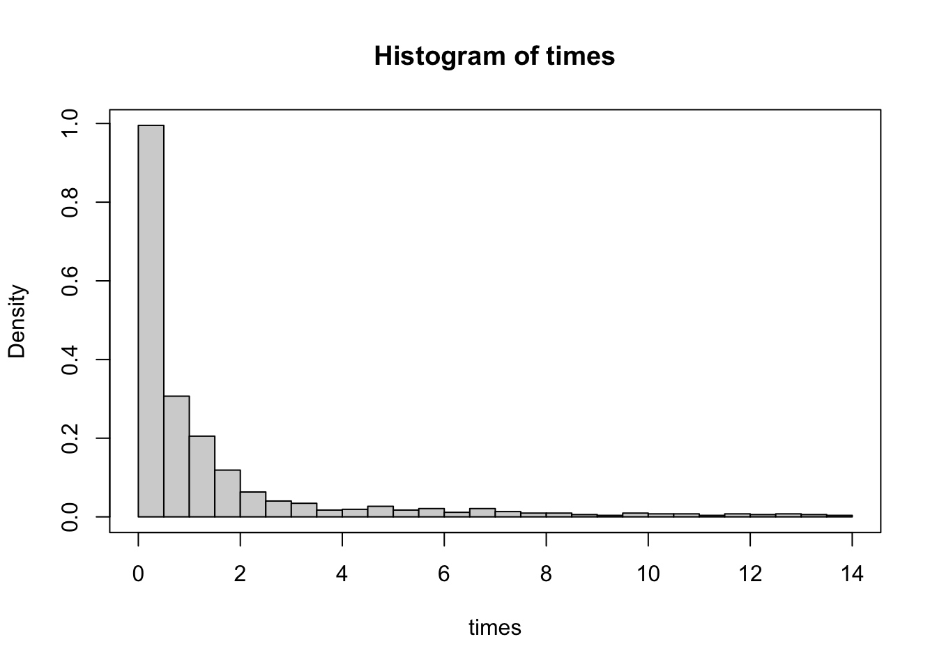
In this example, we analyse the LeukSurv data set from the R package spBayesSurv. This data set contains information about the survival of acute myeloid leukemia in 1,043 patients.

For the GH model, we consider the hazard level covariates (\({\bf x}\)) age (standardised), sex, wbc (white blood cell count at diagnosis, standardised), and tpi (the Townsend score, standardised); and the time level covariates (\({\bf x}\)) age (standardised), wbc (white blood cell count at diagnosis, standardised), and tpi (the Townsend score, standardised). For the PH, AFT, and AH models, we consider the covariates age (standardised), sex, wbc (white blood cell count at diagnosis, standardised), and tpi (the Townsend score, standardised).

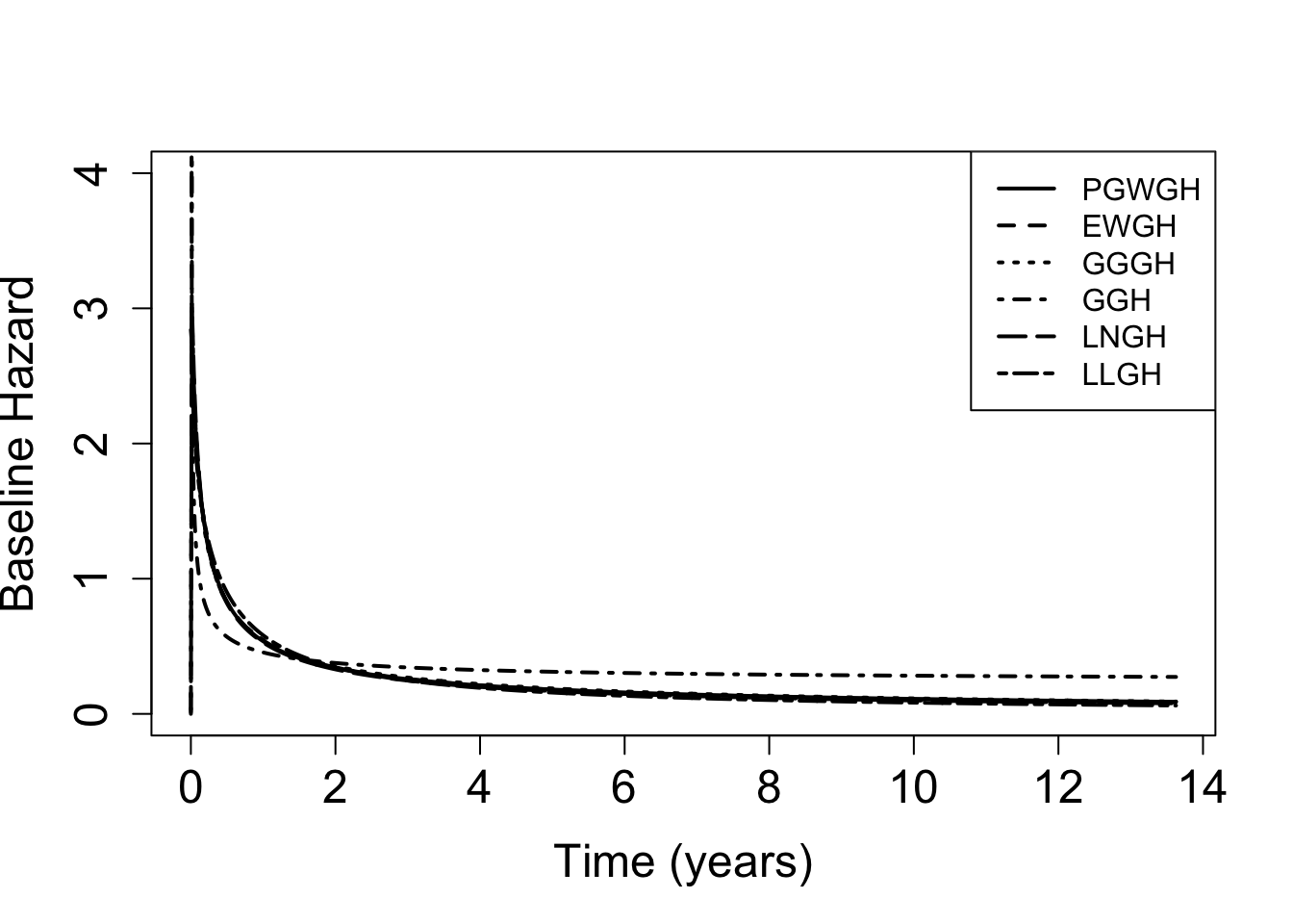
For illustration, we fit the 4 models with both (3-parameter) PGW and (2-parameter) LL baseline hazard. In addition, we fit the GH model with GG, EW, LN, and G baseline hazards. We compare these models in terms of AIC (BIC can be used as well). We summarise the best selected model with the available tools in this package.

See also: GHSurv, LBANS

3.1 Data preparation

Code
rm(list=ls())

# Required packages
#library(devtools)
#install_github("FJRubio67/HazReg")
library(HazReg)
library(numDeriv)
library(spBayesSurv)
library(knitr)
library(survival)
library(mvtnorm)

# Data
data(LeukSurv)

# Design matrix for hazard level effects
X <- as.matrix(cbind(scale(LeukSurv$age), LeukSurv$sex, scale(LeukSurv$wbc), scale(LeukSurv$tpi) ))

# Design matrix for time level effects
Xt <- as.matrix(cbind(scale(LeukSurv$age), scale(LeukSurv$wbc), scale(LeukSurv$tpi)))

# Vital status
status <- as.vector(LeukSurv$cens)

# Survival times
times <- as.vector(LeukSurv$time)/365.24 # in years

# Histogram of survival times
hist(times, probability = TRUE, breaks = 30)
box()

3.2 Model fit and MLEs

Code
# PGWGH
OPTPGWGH <- GHMLE(init = rep(0, 3 + ncol(X) + ncol(Xt)), times = times, status = status, 
                   hstr = "GH", dist = "PGW", des = X, des_t = Xt, method = "nlminb", maxit = 10000)

# PGWAFT
OPTPGWAFT <- GHMLE(init = rep(0, 3 + ncol(X)), times = times, status = status, 
                    hstr = "AFT", dist = "PGW", des = X, method = "nlminb", maxit = 10000)

# PGWPH
OPTPGWPH <- GHMLE(init = rep(0, 3 + ncol(X)), times = times, status = status, 
                   hstr = "PH", dist = "PGW", des = X, method = "nlminb", maxit = 10000)

# PGWAH
OPTPGWAH <- GHMLE(init = rep(0, 3 + ncol(X)), times = times, status = status, 
                   hstr = "AH", dist = "PGW", des_t = X, method = "nlminb", maxit = 10000)


# LLGH
OPTLLGH <- GHMLE(init = rep(0, 2 + ncol(X) + ncol(Xt)), times = times, status = status, 
                 hstr = "GH", dist = "LogLogistic", des = X, des_t = Xt, method = "nlminb", maxit = 10000)

# LLAFT
OPTLLAFT <- GHMLE(init = rep(0, 2 + ncol(X)), times = times, status = status, 
                  hstr = "AFT", dist = "LogLogistic", des = X, method = "nlminb", maxit = 10000)

# LLPH
OPTLLPH <- GHMLE(init = rep(0, 2 + ncol(X)), times = times, status = status, 
                 hstr = "PH", dist = "LogLogistic", des = X, method = "nlminb", maxit = 10000)

# LLAH
OPTLLAH <- GHMLE(init = rep(0, 2 + ncol(X)), times = times, status = status, 
                 hstr = "AH", dist = "LogLogistic", des_t = X, method = "nlminb", maxit = 10000)


# EWGH
OPTEWGH <- GHMLE(init = rep(0, 3 + ncol(X) + ncol(Xt)), times = times, status = status, 
                 hstr = "GH", dist = "EW", des = X, des_t = Xt, method = "nlminb", maxit = 10000)

# GGGH
OPTGGGH <- GHMLE(init = rep(0, 3 + ncol(X) + ncol(Xt)), times = times, status = status, 
                 hstr = "GH", dist = "GenGamma", des = X, des_t = Xt, method = "nlminb", maxit = 10000)

# LNGH
OPTLNGH <- GHMLE(init = rep(0, 2 + ncol(X) + ncol(Xt)), times = times, status = status, 
                 hstr = "GH", dist = "LogNormal", des = X, des_t = Xt, method = "nlminb", maxit = 10000)

# GGH
OPTGGH <- GHMLE(init = rep(0, 2 + ncol(X) + ncol(Xt)), times = times, status = status, 
               hstr = "GH", dist = "Gamma", des = X, des_t = Xt, method = "nlminb", maxit = 10000)

# MLEs in the original parameterisations
MLEPGWGH <- c(exp(OPTPGWGH$OPT$par[1:3]),OPTPGWGH$OPT$par[-c(1:3)])
MLEEWGH <- c(exp(OPTEWGH$OPT$par[1:3]),OPTEWGH$OPT$par[-c(1:3)])
MLEGGGH <- c(exp(OPTGGGH$OPT$par[1:3]),OPTGGGH$OPT$par[-c(1:3)])
MLEGGH <- c(exp(OPTGGH$OPT$par[1:2]),OPTGGH$OPT$par[-c(1:2)])
MLELNGH <- c(OPTLNGH$OPT$par[1], exp(OPTLNGH$OPT$par[2]), OPTLNGH$OPT$par[-c(1,2)])
MLELLGH <- c(OPTLLGH$OPT$par[1], exp(OPTLLGH$OPT$par[2]), OPTLLGH$OPT$par[-c(1,2)])

MLES <- cbind(MLEPGWGH, MLEEWGH, MLEGGGH, c(MLEGGH[1:2], NA, MLEGGH[-(1:2)]), 
              c(MLELNGH[1:2], NA, MLELNGH[-(1:2)]), c(MLELLGH[1:2], NA, MLELLGH[-(1:2)]))
colnames(MLES) <- c("PGWGH", "EWGH", "GGGH", "GGH", "LNGH", "LLGH")
rownames(MLES) <- c("theta[1]","theta[2]","theta[3]","age_t","wbc_t","tpi_t","age", "sex","wbc","tpi")

# MLEs for GH models
# theta[1] in GGGH < 0.001, which is the reason why the rounded value appears as 0.000
kable(MLES, digits = 3)
PGWGH EWGH GGGH GGH LNGH LLGH
theta[1] 0.095 0.006 0.000 0.488 -0.730 -0.718
theta[2] 1.006 0.219 3.105 4.118 1.981 1.126
theta[3] 3.474 8.957 0.086 NA NA NA
age_t 0.911 0.886 0.898 -0.800 0.853 0.828
wbc_t 0.898 0.847 0.861 -0.511 0.788 0.741
tpi_t 0.413 0.407 0.439 -0.592 0.370 0.420
age 0.979 0.969 0.971 0.338 0.958 0.949
sex 0.077 0.071 0.066 0.148 0.074 0.072
wbc 0.681 0.656 0.658 0.004 0.630 0.609
tpi 0.303 0.302 0.315 -0.115 0.287 0.315

3.3 Model Comparison

Code
# AIC for models with PGW baseline hazard
AICPGWGH <- 2*OPTPGWGH$OPT$objective + 2*length(OPTPGWGH$OPT$par)
AICPGWAFT <- 2*OPTPGWAFT$OPT$objective + 2*length(OPTPGWAFT$OPT$par)
AICPGWPH <- 2*OPTPGWPH$OPT$objective + 2*length(OPTPGWPH$OPT$par)
AICPGWAH <- 2*OPTPGWAH$OPT$objective + 2*length(OPTPGWAH$OPT$par)

# AICs for models with LL baseline hazard
AICLLGH <- 2*OPTLLGH$OPT$objective + 2*length(OPTLLGH$OPT$par)
AICLLAFT <- 2*OPTLLAFT$OPT$objective + 2*length(OPTLLAFT$OPT$par)
AICLLPH <- 2*OPTLLPH$OPT$objective + 2*length(OPTLLPH$OPT$par)
AICLLAH <- 2*OPTLLAH$OPT$objective + 2*length(OPTLLAH$OPT$par)

# AICs for GH models with GG, EW, LN, and G hazards
AICGGGH <- 2*OPTGGGH$OPT$objective + 2*length(OPTGGGH$OPT$par)
AICEWGH <- 2*OPTEWGH$OPT$objective + 2*length(OPTEWGH$OPT$par)
AICLNGH <- 2*OPTLNGH$OPT$objective + 2*length(OPTLNGH$OPT$par)
AICGGH <- 2*OPTGGH$OPT$objective + 2*length(OPTGGH$OPT$par)


# All AICs
AICs <- c(AICPGWGH, AICPGWAFT, AICPGWPH, AICPGWAH,
          AICLLGH, AICLLAFT, AICLLPH, AICLLAH,
          AICGGGH, AICEWGH, AICLNGH, AICGGH)

round(AICs, digits = 2)
 [1] 1537.24 1539.48 1586.48 1628.54 1527.41 1529.38 1580.56 1664.46 1534.76
[10] 1533.73 1533.68 1705.96
Code
# Best model: LLGH
which.min(AICs)
[1] 5

3.4 Baseline hazards for GH models

Code
# Fitted baseline hazard functions for GH models
PGWGHhaz <- Vectorize(function(t) hpgw(t, MLEPGWGH[1], MLEPGWGH[2], MLEPGWGH[3]) ) 
EWGHhaz <- Vectorize(function(t) hew(t, MLEEWGH[1], MLEEWGH[2], MLEEWGH[3]) ) 
GGGHhaz <- Vectorize(function(t) hggamma(t, MLEGGGH[1], MLEGGGH[2], MLEGGGH[3]) ) 
GGHhaz <- Vectorize(function(t) hgamma(t, MLEGGH[1], MLEGGH[2]) ) 
LNGHhaz <- Vectorize(function(t) hlnorm(t, MLELNGH[1], MLELNGH[2])) 
LLGHhaz <- Vectorize(function(t) hllogis(t, MLELLGH[1], MLELLGH[2])) 

# Note that the baseline hazards associated to the top models look similar
curve(PGWGHhaz,1e-6, max(times), xlab = "Time (years)", ylab = "Baseline Hazard", main = "",
      cex.axis = 1.5, cex.lab = 1.5, lwd = 2, ylim = c(0,4), n = 1000)
curve(EWGHhaz,1e-6, max(times), lwd = 2, n = 1000, lty = 2, add = TRUE) 
curve(GGGHhaz,1e-6, max(times), lwd = 2, n = 1000, lty = 3, add = TRUE) 
curve(GGHhaz,1e-6, max(times), lwd = 2, n = 1000, lty = 4, add = TRUE) 
curve(LNGHhaz,1e-6, max(times), lwd = 2, n = 1000, lty = 5, add = TRUE) 
curve(LLGHhaz,1e-6, max(times), lwd = 2, n = 1000, lty = 6, add = TRUE) 
legend("topright", legend = c("PGWGH", "EWGH", "GGGH", "GGH", "LNGH", "LLGH"), lwd = rep(2,6), lty = 1:6)

3.5 Best-model summaries

Code
# MLE in the original parameterisation
MLE <- c(OPTLLGH$OPT$par[1], exp(OPTLLGH$OPT$par[2]), OPTLLGH$OPT$par[-c(1,2)])

round(MLE, digits = 3)
[1] -0.718  1.126  0.828  0.741  0.420  0.949  0.072  0.609  0.315
Code
# 95% Confidence intervals under the reparameterisation
CI <- Conf_Int(FUN = OPTLLGH$log_lik, MLE = OPTLLGH$OPT$par, level = 0.95)
rownames(CI) <- c("theta[1]","theta[2]","age_t","wbc_t","tpi_t","age", "sex","wbc","tpi")

kable(CI, digits = 3)
Lower Upper Transf MLE Std. Error
theta[1] -0.884 -0.553 -0.718 0.084
theta[2] 0.060 0.177 0.119 0.030
age_t 0.528 1.128 0.828 0.153
wbc_t 0.492 0.989 0.741 0.127
tpi_t 0.120 0.720 0.420 0.153
age 0.791 1.107 0.949 0.081
sex -0.058 0.202 0.072 0.066
wbc 0.446 0.773 0.609 0.083
tpi 0.149 0.481 0.315 0.085
Code
# Fitted baseline hazard function
fit_haz <- Vectorize(function(t) hllogis(t, MLE[1], MLE[2])) 

curve(fit_haz,0.001, max(times), xlab = "Time (years)", ylab = "Baseline Hazard", main = "",
      cex.axis = 1.5, cex.lab = 1.5, lwd = 2, ylim = c(0,4), n = 1000)

Code
# Average population survival function and KM estimator

pop_surv <- Vectorize(function(t){
  p0 <- dim(Xt)[2]
  p1 <- dim(X)[2]
  theta1 <- MLE[1]; theta2 <- MLE[2]; alpha <- MLE[3:(2+p0)]; beta <- MLE[(3+p0):(2+p0+p1)]
  x.alpha <- Xt%*%alpha
  x.dif <- X%*%beta - x.alpha
  out <- mean( exp( - chllogis(t*exp(x.alpha), theta1, theta2)*exp(x.dif)  )  )
  return(out)
})


# Kaplan-Meier estimator 
km <- survfit(Surv(times, status) ~ 1)

# Comparison
plot(km$time, km$surv, type = "l", col = "black", lwd = 2, lty = 1, ylim = c(0,1),
     xlab = "Time (years)", ylab = "Population Survival", main = "",
     cex.axis = 1.5, cex.lab = 1.5)
curve(pop_surv,0.001,14, lwd = 2, n = 1000, add = TRUE, lty = 2, col = "gray")
legend("topright", legend = c("KM","Parametric"), col = c("black","gray"), lwd = c(2,2), lty = c(1,2))

Code
# Confidence intervals for the survival function based on a normal approximation
# at specific time points t0

# Hessian and asymptotic covariance matrix
HESS <- hessian(func = OPTLLGH$log_lik, x = OPTLLGH$OPT$par)
Sigma <- solve(HESS)

# Reparameterised MLE 
r.MLE <- OPTLLGH$OPT$par

# The function to obtain approximate CIs based on Monte Carlo simulations 
# from the asymptotic normal distribution of the MLEs
# t0 : time where the confidence interval will be calculated
# level : confidence level
# n.mc : number of Monte Carlo iterations

conf.int.surv <- function(t0, level, n.mc){
  p0 <- dim(Xt)[2]
  p1 <- dim(X)[2]
  mc <- vector()
  S.par <- function(par){ mean( exp( - chllogis(t0*exp(Xt%*%par[3:(2+p0)]), par[1], par[2])*
                                      exp(X%*%par[(3+p0):(2+p0+p1)]-Xt%*%par[3:(2+p0)])  )  )
  }
  
  for(i in 1:n.mc) {
    val <- rmvnorm(1,mean = r.MLE, sigma = Sigma)
    val[2] <- exp(val[2])
    mc[i] <- S.par(val)
  }
  
  L <- quantile(mc,(1-level)*0.5)
  U <- quantile(mc,(1+level)*0.5)
  
  M <- S.par(MLE)
  
  return(c(L,M,U))
}


# times for CIs calculations
timesCI <- c(1,2.5,5,7.5,10,12.5)

CIS <- matrix(0, ncol = 4, nrow = length(timesCI))

for(k in 1:length(timesCI)) CIS[k,] <- c(timesCI[k],conf.int.surv(timesCI[k],0.95,10000))

colnames(CIS) <- cbind("year","lower","population survival","upper")
print(kable(CIS,digits=4))


| year|  lower| population survival|  upper|
|----:|------:|-------------------:|------:|
|  1.0| 0.3360|              0.3568| 0.3798|
|  2.5| 0.2013|              0.2191| 0.2403|
|  5.0| 0.1279|              0.1428| 0.1611|
|  7.5| 0.0951|              0.1089| 0.1263|
| 10.0| 0.0770|              0.0892| 0.1057|
| 12.5| 0.0644|              0.0761| 0.0917|

References

Chen, Y. Q., and N. P. Jewell. 2001. “On a General Class of Semiparametric Hazards Regression Models.” Biometrika 88 (3): 687–702.
Chen, Y. Q., and M. C. Wang. 2000. “Analysis of Accelerated Hazards Models.” Journal of the American Statistical Association 95 (450): 608–18.
Cox, D. R. 1972. “Regression Models and Life-Tables.” Journal of the Royal Statistical Society: Series B (Methodological) 34 (2): 187–202.
Kalbfleisch, J. D., and R. L. Prentice. 2011. The Statistical Analysis of Failure Time Data. John Wiley & Sons.
Rubio, F. J., L. Remontet, N. P. Jewell, and A. Belot. 2019. “On a General Structure for Hazard-Based Regression Models: An Application to Population-Based Cancer Research.” Statistical Methods in Medical Research 28: 2404–17.